TAG_TSEMA - Tutorial |
|
This short tutorial is intended for you to get familiar with TAG_TSEMA's interface and with some concepts used during the process of obtaining and refining a mapping.
Let's start with one of the examples available in the server. This is a toy example in the sense that the mapping between the leaves of both trees is known. This trivial mapping is given by the organism relationships since the two interacting families are families of orthologs. The two families contains the orthologs of two E coli proteins known to interact: Ribonucleoside-diphosphate reductase 1 beta (P00453) and alpha (P00452) subunits. The (trivial) correct mapping would be P00453 of E coli with P00452 of E coli, P00453 of H pylori with P00452 of H pylori, and so forth.
To "predict" the mapping between these two families based on tree similarity, you can run TAG_TSEMA with the trees of both families. In the "Examples" page, you can get these trees (generated by neighbour joining) in newick format (.ph). You can also use as input the multiple sequence alignments (.pir). In this case, TAG_TSEMA would generate the trees with the neighbour joining algorithm implemented in ClustalW. You can try to generate your own trees using more sophisticated algorithms (parsimony or bayesian trees) from the multiple sequence alignments (.pir), use them as input for the server, and compare the results.
Download the trees (.ph) of both families to your hard disk. Then go to the "New Job" section and upload these files in the "Tree/MSA for Family I" and "Tree/MSA for Family II" boxes. Additionally, provide a name for the job and an email address in the corresponding text-boxes. Press "Submit" to start the job.
Internally, the system is going to run 500 non-exhaustive explorations of the space of solutions (mappings) using a modified implementation of Ramani & Marcotte's Montecarlo-based approach. In each one of these 500 Montecarlo runs, a maximum of 10 million mappings is explored. The default scoring function for evaluating the goodness a mapping is is Pearson's T score. You might change some of these parameters enabling "advanced options".
After completion of the job, you receive by email a .tar.gz file with all the results. Apart from other information, this file contains the best trees found in each one of the 500 runs. Advanced users can use that raw file as it is and process it using their own methods. Save this file taking care that the file extension remains as ".tar.gz" (some operative systems try to change it). That file is also available in the "Examples" page and you can start from it if you do not want to do the previous part. Note that, due to the intrinsic stochastic nature of the process, the results can be slightly different from one experiment to another and to the results stored in the "Examples" page. This tutorial was done with the file in the "Examples" page.
To interactively analyze and modify the raw results of the Montecarlo step, upload the .tar.gz file with the raw results in the "Results file" box of the "New Analysis" page (It is NOT compulsory to provide a job name and an email in this page.) Then press "Submit".
In the interactive analysis page, you can see the list of predicted pairs according with the overall best mapping (the best of the 500).
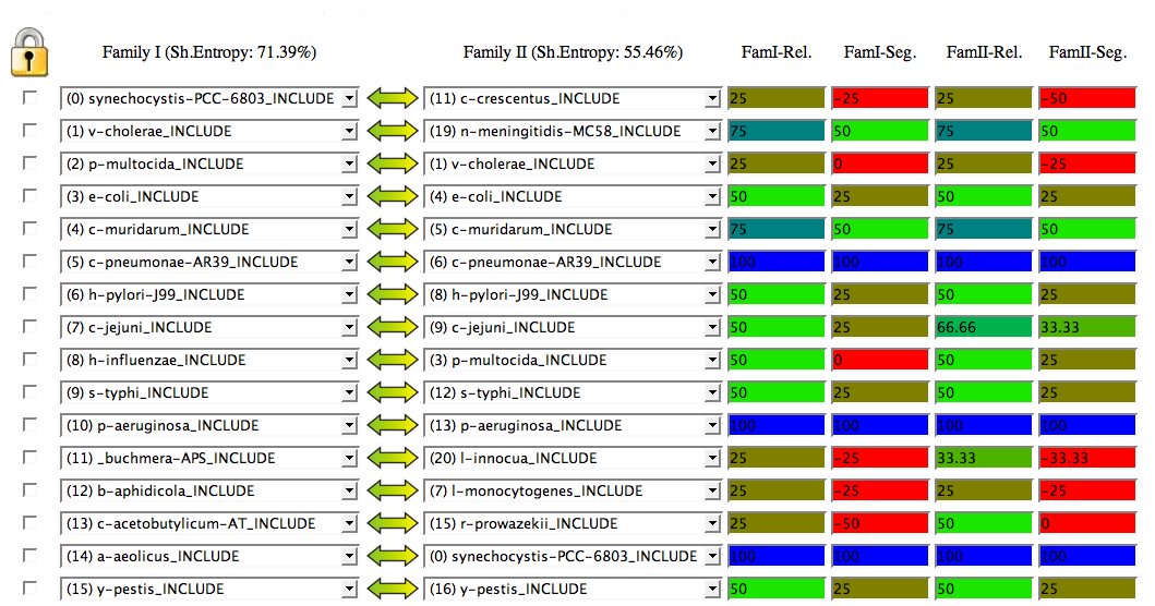
At the top of this list, you can see the entropies of both trees (in a 0-100 scale). Entropy is an indicator of the complexity of the tree, the amount of information it has and that can be used to find the best mapping with the other tree. Basically, it is a measure of how rich is the range of distances it contains. Imagine a "star" tree with all the proteins at the same distance from each other (entropy=0). It would be impossible to find the right mapping with other trees since all the mappings would be topologically indistinguishable and would have the same score. So, better results are expected for trees with high entropies.
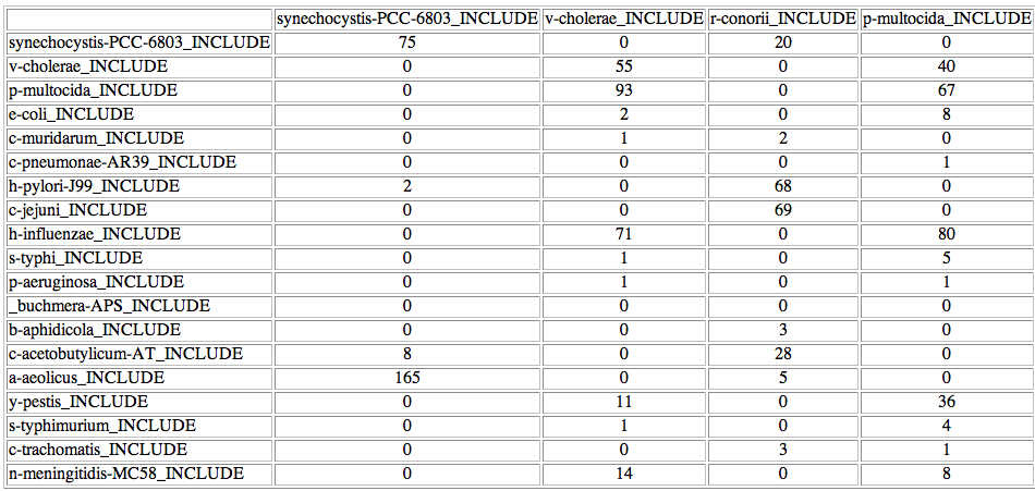
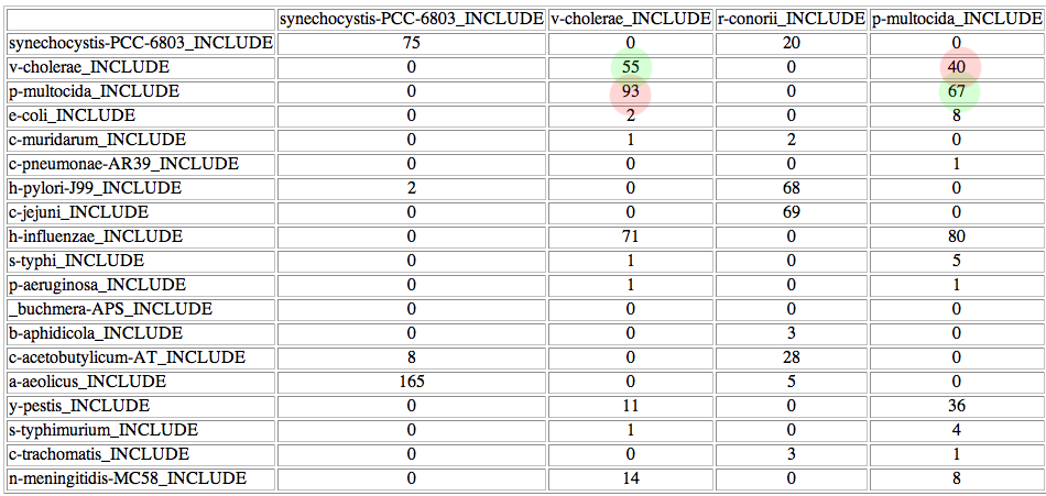
At the bottom of the list there is a button to access the "coincidence matrix". This matrix shows, for each possible pair of proteins, in how many of the 500 best trees that pair is present. For example, in this case synechocystis-PCC-6803 is linked with synechocystis-PCC-6803 in 75 of the 500 trees, while it is linked to r-conorii in 20, etc.
For each pair, 4 scores are calculated from this coincidence matrix:
The Reliability score for a pair A-B (Rel) indicates in how many of the 500 trees A is linked to B over the total number of pairings for A (in percentage). The Segregation score (Seg) for a pair gives an idea of the difference between the Reliability of that pair and the next best reliability. There is a color scale for these two scores, from red (worst) to blue (best).
Take a look at the Help page for a better description of these two scores.
The next section of the screen shows a representation of the two phylogenetic trees including the links corresponding to the best mapping. The color of the links corresponds to the Rel_AB.
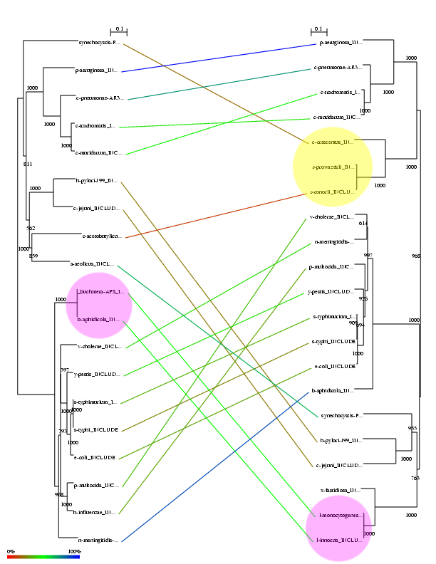
It can be seen that most of the links between the two interacting families proposed by the system are right. Most of false positives are due to organisms which are not present in one of the families. For example, the protein on the right is not present in the clade of three organisms marked in yellow. The system incorrectly matches two of these organisms with two organisms on the left. In this case the score for these links is low (red and brown colors) reflecting that these links are not consistent. A more difficult case is the two pairs of organisms marked with pink color. The sequences of both proteins within these two pairs are 100% identical (distance=0 in the tree). The system links these proteins consistently (good score, green). This shows that, in a real example, the user should exclude 100% identical proteins since it is topologically impossible for the algorithm to distinguish them. Related with that, proteins at similar distances from their ancestor produce very similar sets of distances and hence they are difficult to distinguish. See for example the pair C trachomatis / C muridarum. In the best solution, the correct pairings are swapped.
The coincidence matrix is a good starting point for trying some mappings not explored by the heuristic approach. For example, the organisms V cholerae and P multocida are incorrectly paired. It can be seen in the coincidence matrix that the right pairings are also very common within the 500 best solutions:
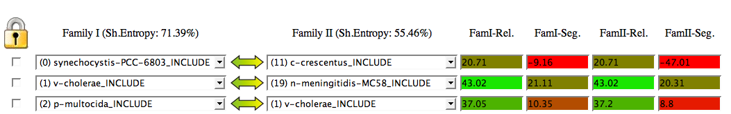
In a real test, the user should try these pairings suggested by the coincidence matrix. In this case, you should change the predicted interactor for V cholerae (N meningitidis) and try V cholerae based on the coincidence matrix The results suggest that you should do the same for P multocida. Please notice that whenever a change is made the new mapping incorporating your changes is represented. You can see that the score has been slightly improved after those changes. The solution (mapping) you are seeing has a better score than the original one and it has two more real interacting pairs. It was not been explored by the Montecarlo approach due to its stochastic nature.